Using MOE, the Metric Optimization Engine, to Optimize an A/B Testing Experiment Framework

-
Dr. Scott Clark, Ad Targeting Engineer
- Oct 9, 2014
A/B Testing Experiment Frameworks and MOE
We recently open sourced MOE, the Metric Optimization Engine, a machine learning tool for solving global, black box optimization problems. An example application for such a system is optimally running online A/B experiments.
A/B testing segments the users that come to a site into buckets, or cohorts, and show different versions of the site to different cohorts of users. One can show 50% of users one version of a site (version A) and 50% of users another version of a site (version B). After some amount of time we can see which version of the site performs better on various metrics (like Click Through Rate (CTR), conversions, or total revenue) and shift all of your traffic over to the better version. This can be repeated as we converge towards the best version of the site under the metric(s).
It can take a long time to attain statistically significant results for experiments. We want to know with high confidence that one version of the site is better than another. Depending on user traffic it can take days, or even weeks, to run a single iteration. These experiments are also expensive; by showing a suboptimal version of your site, you are sacrificing potential revenue. There is also an opportunity cost associated with creating, developing, and running any particular experiment. So the fewer experiment iterations to get to the optimum, the better.
Furthermore, many A/B tests are merely parameter selection problems (an A/A’ test, where a feature stays the same, and only the underlying parameters change). Given a feature, we want to find the optimal configuration values for its parameters as quickly as possible.
MOE was designed to optimally solve problems like this, when we want to find an optimal set of parameters (inputs) of a function (a metric, like CTR) when sampling this function is time consuming or expensive (like running an A/B test experiment on live traffic). By leveraging MOE we can build a general experiments platform that automatically promotes good cohorts and pushes traffic away from under-performing cohorts, then replacing them with new, winning configurations.
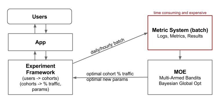
Figure 1: MOE can be used to optimally assign traffic allocations in an A/B testing framework and to suggest new parameters to sample given the historical values already sampled.
Using Multi-Armed Bandits for Optimal Traffic Allocation
Instead of naively allocating traffic in some uniform way (like a 50/50 split) we can use the information about how an individual cohort is performing to dynamically and optimally allocate the best percentage of traffic to it. This is fundamentally a tradeoff between exploration and exploitation. Exploration is equivalent to gaining more knowledge about the system by continuing to allocate traffic to a wide variety of points. Exploitation on the other hand, is using the knowledge we have already gained to get the most expected return out of the system as we currently understand it. Others have shown that using Multi-Armed Bandits can achieve better results, faster, in online A/B tests.
MOE has many different bandit policies implemented and allows the user to select a policy that best fits their desired trade-off between the exploration and exploitation of the data. By using a Multi-Armed Bandit approach we can limit the amount of suboptimal traffic allocation in an A/B test, leaving as few gains on the table as possible.
Using Bayesian Global Optimization to Suggest Parameters
As the Multi-Armed Bandit system starts lowering the traffic allocation for a certain experiment we have two choices. We can turn off that cohort, and allow the remaining cohorts to battle it out until we have one clear winner (within whatever confidence we desire). Alternatively, we can have MOE suggest a new cohort using Bayesian Global Optimization (with a new set of underlying parameters) for the system to try. This allows the system to play an internal game of king-of-the-hill, where better and better parameters are being sampled as the objective continues to rise higher and higher.
MOE uses the historical data gained so far to decide which points to sample next. It suggests new parameters to try that have the highest Expected Improvement under a Gaussian Process model. These are the parameters that are expected beat the current best set of parameters by the most, using whatever metric we provide as the objective function. This method converges much faster to global optima than other heuristic methods like grid search, random search or basic hill climbing.
By constantly spinning down underperforming cohorts in our experiment and replacing them with optimal new cohorts we allow our experiment framework to continually search the underlying parameter space for the best possible parameters.
Putting it all Together
Let’s assume that we want to optimize some underlying parameter that affects our ad Click Through Rate (CTR) in some way. This parameter could represent anything from a threshold in our system to some hyperparameter to a feature in our ad targeting system. Let’s say we currently are running with this parameter set to the value 0.2 in production, our status quo.
We would like to run an experiment where we sample other values of parameter in an attempt to maximize CTR. We will need to run time consuming and expensive experiments every time we want to measure CTR, so we will use MOE to help us find the optimal value in as few samples as possible. We simulate the observed CTR of the system for 1 million users by sampling from a Bernoulli distribution with the given true CTR.
In a real world system we do not know exactly how the underlying parameter affects CTR, which is why we need to sample various values with real traffic to find the optima. For the purposes of this example, we will define the exact function of CTR with respect to the underlying parameter for simulation purposes, keeping it hidden from MOE. Note that the function need not be convex or even continuous.
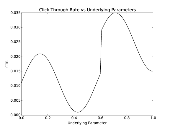
Figure 2: The graph of the true CTR vs the underlying parameter. There is a local CTR maximum at 0.143 and a global CTR maximum at 0.714.
We begin the experiment by asking MOE for 2 new parameter values to sample, in addition to our current status quo value of 0.2. We will set our objective function for MOE to optimize to be the relative gain over the status quo CTR. We note that this gives our status quo parameter a value of 0, and any parameter that has a higher CTR than the status quo will have a positive value, while any parameter that has a lower CTR will have a negative value.
Our initial representation of the underlying system, and the Gaussian Process, looks like Figure 3.
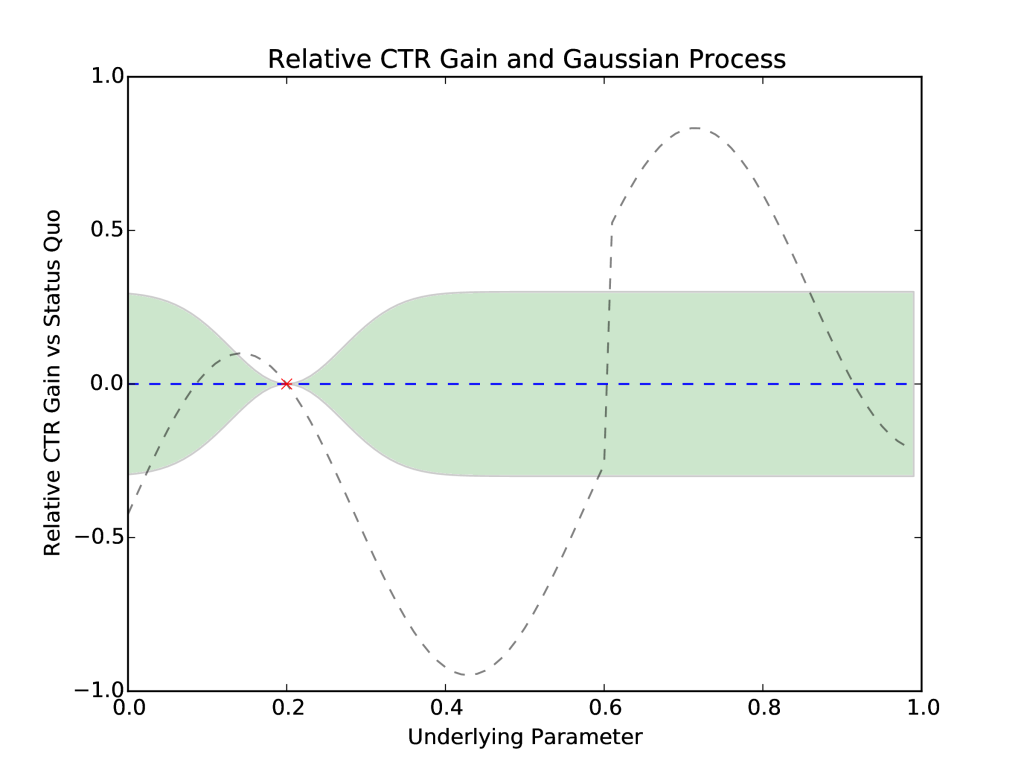
Figure 3: The blue (mean) and green (variance) plot is the initial Gaussian Process representation of the space that MOE optimizes. The dashed gray line is the true, unknown objective function, the relative CTR gain vs status quo.
MOE suggests two points as the initial parameters to test. These will be the corresponding parameters for cohort 1 and cohort 2 respectively. Initially we will conservatively allocate new cohorts to have 5% of traffic each, using the epsilon greedy bandit policy with epsilon set to 0.15. The remaining 90% of traffic will go towards the best parameter value observed so far.
Once we have the simulated data we can determine which cohorts have performed well and which ones should be turned off. We turn off any cohort that has a CTR more than two standard deviations worse than the current best observed CTR. We then query MOE for new, optimal parameters to sample given how all historical parameters have performed. This is repeated multiple times as poorly performing parameter values are culled and new parameter values are suggested by MOE. See Figure 4 for the evolution of the underlying Gaussian Process and watch MOE converge to the globally optimal parameter value.

Figure 4: The new points be sampled each day (red x) and previous points (blue x) influence the Gaussian Process representation of the relative CTR gain that MOE uses to optimize the underlying parameter. We can see the Gaussian Process getting more accurate with respect to the true function (dashed gray) as more points are sampled.
By iterating to the global optimal parameter value in as few samples as possible, we can increase the system CTR far beyond the initial status quo value, or even the local maxima. In this example, by the second set of sampled parameters MOE is beating both the status quo CTR value and the CTR the best local parameter value, achieving the best global parameter value within the third set of sampled points.
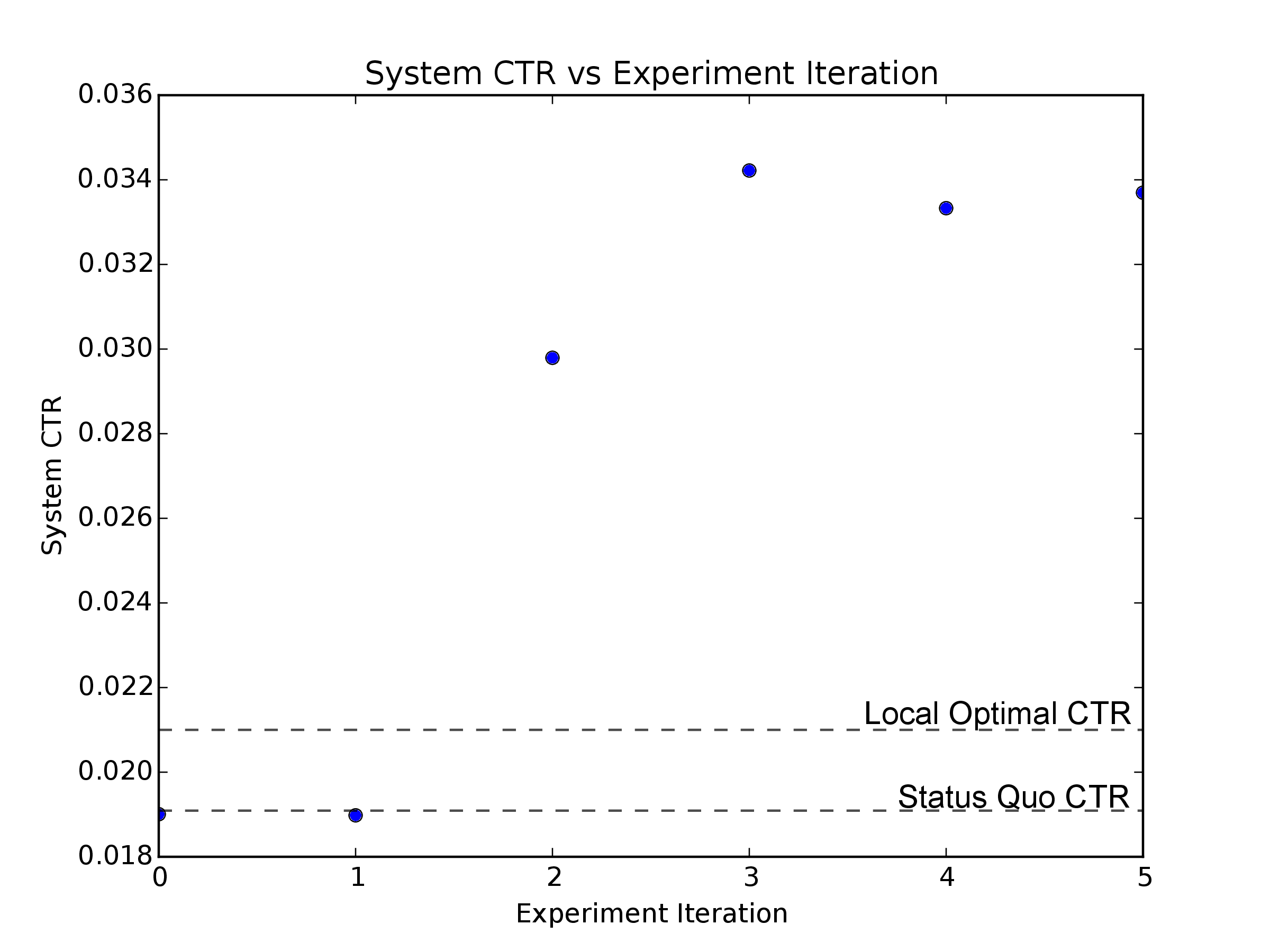
Figure 5: The simulated CTR during for each round of sampled parameter values. Initially the system CTR is equal to the status quo CTR. MOE quickly finds better and better values of the underlying parameter, converging to the global optima in 3 short sets of samples.
Using MOE in your experiment framework
- All of the code used to generate this example can be found here.
- Other examples of using MOE can be found here.
- The Multi-Armed Bandit portion of MOE is documented here.
- The Bayesian Global Optimization components are documented here.
- Any issues can be reported in the issue tracker.
- Questions or comments can be sent to opensource+moe@yelp.com.