Accelerating Retention Experiments with Partially Observed Data

-
Conner DiPaolo, Applied Scientist
- Feb 20, 2020
Summary
Here at Yelp, we generate business wins and a better platform by running A/B tests to measure the revenue impact of different user and business experience interventions. Accurately estimating key revenue indicators, such as the probability a customer retains at least \(n\)-days (\(n\)-day retention) or the expected dollar amount a customer spends over their first \(n\) days (\(n\)-day spend) is core to this experimentation process.
Historically at Yelp, \(n\)-day customer or user retention was typically estimated as the proportion of customers/users we observed for more than \(n\) days who retained more than \(n\) days. Similarly, \(n\)-day spend was estimated as the average amount spent over the first \(n\) days since experiment cohorting by businesses we have observed for at least \(n\) days.
Recently, we transitioned to using two alternative statistical estimators for these metrics: the Kaplan-Meier estimator and the mean cumulative function estimator. These new approaches consider censored data, i.e. partially observed data, like how long a currently subscribed advertiser will retain as a customer. Accordingly, they offer several benefits over the previous approaches, including higher statistical power, lower estimate error, and more robustness against within-experiment seasonality.
By performing Monte-Carlo simulations [1, Chapter 24], we determined that using these estimators allowed us to read A/B experiment metrics a fixed number of days earlier after cohorting ends without any drop in statistical power. This amounted to a 12% to 16% reduction in overall required cohorting and observation time, via a 25% to 50% reduction in the time used to observe how people respond to the A/B experiences. Altogether, this improved our ability to iterate on our product.
Background: Revenue Experimentation at Yelp
The value of a Yelp customer can be quantified in two primary and informative directions: how long a user / business remains active / subscribed in our system (known as retention), as well as the total dollar amount they generate over their lifetime (known as cumulative spend). When we experiment on different user / business experiences, we make a point of estimating the effect of these changes on retention and spend metrics before we make a final ship decision.
As a proxy, sometimes dollars might be replaced with less noisy units like ad clicks, page views, etc., but for the purposes of this blog post we will focus on altering a business experience and analyzing \(n\)-day retention and spend. The conclusions carry over equally well to experimentation settings that either deal with users or with similarly defined proxy metrics.
The diagram below illustrates the typical lifecycle of an A/B test focused on retention and spend.
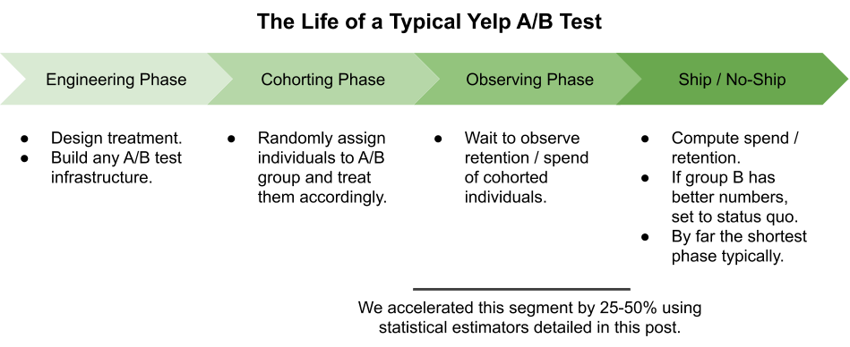
Depending on the type of experience change and the time window used for measurement, the cohorting and observing phases can in many instances take the most time of the whole experimentation pipeline. As such, the acceleration of the observing phase detailed here can provide improvements in our ability to iterate on our product.
Uncensored Approaches To Computing Retention & Spend
One possible retention measure is “what percentage of those in cohort \(C\) who subscribed to product \(P\) at any point during the experiment went on to retain for more than \(n\) days,” where \(C\), \(P\), and \(n\) are parameters the experimenter can adjust. Yelp previously computed this \(n\)-day retention measure within each experiment cohort as follows: of the customers who started purchasing product \(P\) during the experiment who we have observed for at least \(n\) days since their initial purchase, report the proportion who are still subscribed at day \(n\).
Our measure for dollars spent is analogous: we measure \(n\)-day spend by considering “on average, how many dollars do those in cohort \(C\) spend on products \(P_1, P_2, \ldots, P_k\) over their first \(n\) days after being cohorted.” Here, \(C\), the product basket \(P_1, P_2, \ldots, P_k\), and \(n\) are freely adjustable as above.
Standard error estimates for both of these metric estimators which rely on the Central Limit Theorem are always reported as well [1, Theorem 6.16]. These estimators are unbiased and consistent (as the number of people observed for at least \(n\) days grows), assuming that the retention of customers is independent of the relative time they enter the experiment.
There are a number of potential concerns that can arise from using the estimators mentioned above.
Variance: One of the greater concerns is that estimators could have large variance if only a small number of customers had been observed in a cohort during the experiment period. Let’s suppose we want to cohort individuals into an experiment for 70 days and are interested in estimating the 60-day retention of each cohort in the experiment. At day 75, the uncensored estimators above only access the users who arrived during the first 15 days of experiment cohorting, even though we have been cohorting users for 5 times as long. Therefore, unless the sample size is very large or the underlying retention/spend distribution is very concentrated, our estimator will have large variance at this point. This forces us to wait more days after the experiment ends to get a genuine metric read or detect a bona-fide difference in retention or spend of the cohorts.
Seasonality: In addition to the variance issue, the retention or spend characteristics of individuals cohorted into an experiment may vary with the experiment runtime. In this situation, the uncensored estimators will in general be biased away from the true population mean retention and spend over the experiment window until after the observation phase is fully completed. For example, if we run a revenue experiment that starts right before Christmas, the 60-day retention estimate 75 days after the hypothetical experiment above was started would be heavily biased towards HVAC contractors and retail stores instead of the large fraction of restaurants that were closed over the holidays. It is feasible that we could declare a difference between the two populations at day 75 and make a conclusion about the experiment results, even though the underlying estimates are biased and reflect only a subset of the population.
The Kaplan-Meier Estimator for Retention
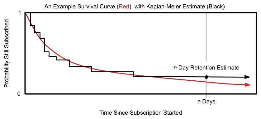
Our solution to a more effective retention estimate, which can mitigate the problems mentioned above, is based on the so-called Kaplan-Meier estimator of the “survival curve.” The survival curve \(S(t)\) is a function of time \(t\) which returns the probability that someone would retain for at least \(t\) days after subscribing. Accordingly, if we had access to the population survival curve, \(S(n)\) would return the proportion of businesses in our population who would retain at least \(n\) days, precisely our retention metric. The Kaplan-Meier estimator is a nonparametric estimator of the whole survival curve. Evaluating the estimated curve at time \(t = n\) days gives an estimate of the desired retention metric:
For a coarser discretization of time than typically used, this Kaplan-Meier estimate of \(n\)-day retention first writes the \(n\)-day churn as \[S(n) = \prod_{t=1}^n \mathrm{Pr}(\text{remains subscribed through day }t |\text{ subscribed for first }t - 1\text{ days}).\] At this point, each multiplicand is estimated as \(h_t\) , the fraction of people we have observed for at least \(t\) days and were subscribed at the end of day \(t - 1\), who then stayed subscribed through the end of day \(t\). The full estimate is then \[S(n) = \prod_{t=1}^n h_t.\] This equals the status quo version that does not incorporate censored data if we instead used the individuals observed for at least \(n\) days to compute each \(h_t\) instead of the larger sample size afforded by using those observed for at least \(t < n\) days. Better utilization of available information can increase the precision of our estimates, increase statistical power to detect differences in cohort retentions, and mitigate sensitivity to time-dependent retention characteristics over the course of the experiment.
This estimator is a consistent estimator of the whole survival curve (computed by varying \(n\)) as both the number of individuals and the length of time we observe each of them increase [2]. It is not, in general, unbiased [3], and is also affected by seasonality in the same way that the status quo estimator is affected, although in simulations seasonality had less of an effect on the estimates than with the status quo approach.
The Mean Cumulative Function for Spend
In the cumulative spend setting, we employed the mean cumulative function estimator detailed in [4]. This mean cumulative function estimator writes the total spend of a business through day \(n\) after cohorting as the sum of the spend on the first day after cohorting, the spend on the second day after cohorting, etc., all the way through the spend on the \(n\)-th day after cohorting. Each day-\(t\) spend is then estimated as the average day-\(t\) spend of people we have seen for at least \(t\) days. Since the sample size used to estimate day-1 spend is usually much greater than that used to estimate day-60 spend, this estimator can achieve greater power than a status quo estimator that restricts the sample in each day-\(t\) spend estimate to only the people observed for all \(n\) days.
This estimator is unbiased, consistent as the number of businesses seen through day \(t\) increases, and has mean squared error no greater than that of the status quo estimator. In the presence of seasonality, this estimator will be biased in the same way the status quo estimator will be, but we observe in practice that it typically has lower mean squared error despite this fact.
The variance of our estimate of expected spend over the \(n\) days following cohorting can be written as follows. Mathematically, if \(s_t\) is the random variable giving the distribution over dollars spent by a business throughout their \(t\)-th day after being cohorted, then the variance of this \(n\)-day spend estimate is \[\sum_{t=1}^{n}\frac{\mathrm{Var}(s_t)}{m_t} + \sum_{t\neq t’} \frac{\mathrm{Cov}(s_t, s_{t’})}{max(m_t, m_{t’})},\] where \(m_t=|\{i:\text{individual }i\text{ observed through day }t\}|\). This can be estimated in practice by plugging in empirical unbiased estimates of \(\mathrm{Var}(s_t)\) and \(\mathrm{Cov}(s_t,s_{t’})\). The covariance terms are summed for all \(t\neq t’\) which are both no more than \(n\). This result is similar to the one presented in [4] but differs in our level of discretization.
Estimator Simulations
In order to realize any acceleration in experimentation under the new estimators, we had to create a policy where experimenters would compute their A/B test metrics using these new estimators earlier than they would under the old, uncensored approaches, all while maintaining a comparable statistical power. Because of a relatively limited number of historical A/B tests with which to evaluate this speed-up empirically, we decided to rely on Monte-Carlo simulation to determine the speed-up to prescribe in practice. Although we ended up going with a simpler policy of reading metrics a fixed number of days earlier, such Monte-Carlo simulation of the speedup could be computed in a bespoke way for each proposed A/B test. This would, in some situations, achieve a much greater speed-up than available under the uniform policy we ended up using, at the expense of complexity.
The Simulation Framework
All of our simulation data are generated according to the following probabilistic model:
An experiment is defined as a collection of initial subscription times \(t \sim \mathrm{Uniform}(0,T \text{ days})\) which arrive uniformly between 0 days and \(T\) days. \(T\) was a pre-set constant that was set to be \(K\) days for spend simulations and \(K+10\) days for retention simulations; these are similar enough (and well within the range of typical experiment fluctuation) that the results should be interpreted identically. Also note that this is the continuous uniform distribution: people can arrive half-way or three-quarters of the way through any given day. Every individual has some underlying mean retention time \(\mu(t)\) which is typically a constant in every scenario except Simulation 3 where \(\mu(t) = T’ + b (2t/T - 1)\) to simulate within-experiment seasonality of revenue characteristics. Given the mean retention time \(\mu(t)\), the retention time \(R\) of a subscriber is exponentially distributed with mean \(μ(t)\), which results in a subscription from time \(t\) to time \(t + R \sim t + \mathrm{Exp}(\text{mean}=\mu(t))\). Moreover, in all but the last spend simulation, the amount that someone spends in a day is precisely a constant times the fraction of a day they were an active subscriber. We don’t include non-subscribers in the spend simulation here; non-subscribers are emulated in the stress test later. For a target sample size \(m\) to collect during the simulated experiment, we independently sample \(m\) such subscriptions to create the experimental data.
For every simulated experiment, we then wish to estimate the \(n\)-day retention/spend at time \(K + T_r\) where the read time \(T_r = 0 \text{ days}, 1 \text{ day}, \ldots,\) etc. since the experiment finished. When measuring retention and spend at time \(T_r\) since the experiment finished, we do not have access to any events (e.g. a subscriber churning) at time later than \(T_r\).
All experiment scenarios and results are averaged over 1000 independent trials in the retention simulations and 1500 independent trials in the spend simulations.
Determining The Speed-up: A Statistical Power Simulation
In this simulation, we generated experimental cohorts according to the above data model under various amounts of cohorted subscribing customers and mean retention times. These retention and sample size characteristics were chosen to run the gamut of experimental data we would expect to see in practice. Then, we matched the cohorts with the same sample size pairwise in order to compute the probability that we could detect (with a \(z\)-test) the bona-fide difference in retention / spend between the two hypothetical A/B experiences the different cohorts would receive. We estimated the \(n\)-day retention probability and \(n\)-day spend at day \(0, 1, \ldots , n\) after the experiment cohorting ended using both the status quo estimator and the Kaplan-Meier / mean cumulative function approaches. We stopped estimating spend and retention at day \(n\) after the end of the experiment because all the data are guaranteed to be uncensored at this point, and accordingly the status quo and proposed estimators coincide exactly.
In all scenarios of interest, the test based on the uncensored approaches have lower statistical power (lower probability of detecting the bona-fide retention difference) than the Kaplan-Meier / mean cumulative function based one where statistically comparable. This is particularly noticeable for moderate sample sizes and moderate differences: in one simulated scenario representative of reality, the status quo based test detects the difference less than half of the time on the day the experiment ends, while the Kaplan-Meier approach succeeds over 80% of the time. In two-thirds of the scenarios tested, the Kaplan-Meier approach succeeds at least 5 percentage points of the time more than the status quo approach the day the experiment ends, and in the majority of those cases the difference is over 10 percentage points.
Looking at the simulations results differently, this can be quantified in terms of accelerating the number of days we need to achieve the same statistical power (within a 1% or similarly small relative tolerance) we would achieve if we computed the status quo estimators at day \(n\) after cohorting ends (the typical time we historically have read retention / spend experiment metrics.) The speed-up we observed for the mean cumulative function (relative to the total time used for cohorting and waiting to read retention and spend) for the various scenarios considered are presented below. The results for retention with the Kaplan-Meier estimator are similar and are not shown here. Note that the intervals of relative speed-ups are not confidence intervals — they are point estimates — but reflect the fact that the total time used to cohort and wait for retention historically has not been fixed and instead varies within a range of \(L\) to \(U\) days. If \(k\) is the number of days earlier we read our metrics, the reported interval is simply \(k / U\) to \(k / L\).
| Relative Speed-up | 0.1% Power Tolerance | 1% Power Tolerance | 2% Power Tolerance |
|---|---|---|---|
| Mean | 20-27% | 25-33% | 28-38% |
| 25th Percentile | 8-11% | 13-18% | 17-22% |
| 50th Percentile | 14-19% | 18-24% | 23-30% |
| 75th Percentile | 32-42% | 43-58% | 46-61% |
To incorporate these estimators across all of Yelp’s experiment analysis, we dictated that individuals should read their experiment metrics with speed-up corresponding to the 50th percentile speed-up we observed in these simulations, under a 0.1% power tolerance as compared to the previous status quo approach. In doing so, under the assumption that our simulations were as representative as we believe, about half of experiment settings would see power no less than 0.1% lower than the status quo approach, but almost all would see power no less than 2% lower than the status quo approach. In light of the marked increase in our ability to iterate on Yelp’s products, this felt like a more-than-fair trade to make. Since in many circumstances the speed-up can be much greater than 12-16% over status quo, bespoke recommendations can and will be made in situations when rapid experimentation is extremely important to Yelp’s bottom line.
Stress Test 1: Robustness against Seasonality
In order to check that our simulations don’t break down in real world scenarios, we ran a number of stress tests that injected more extreme versions of reality into our data generating model, checking that the results largely mirrored what we see with the original data model. We only considered retention in this simulation, and not cumulative spend.
In the first of these stress tests, we consider the case where the average subscriber retention time in a cohort is fixed at some number of days, but where the average retention of an individual varies with respect to when they initially make a purchase during the experiment. Fixing some day-zero bias \(b\), the average retention of an individual is linearly interpolated between \(C + b\) and \(C - b\) over the duration of the experiment in a way such that the population average stays the same. For biases chosen from a predefined set of candidates, we track the bias of the \(n\)-day retention probability estimates made by the status quo and Kaplan-Meier approaches as we re-calculate the metrics after the experiment ends.
The Kaplan-Meier retention estimator has uniformly lower bias than the status quo approach where they are statistically comparable. Indeed, in situations with positive day-zero bias, the bias of the Kaplan-Meier estimator is on the order of 50% of the bias of the status quo approach. Moreover, the bias of the Kaplan-Meier estimator decreases super-linearly with respect to how long we wait to make the measurement, while the bias of the status quo estimator decreases linearly. Here, linearity means that the error is a line with a negative slope. This is different from the typical use of “linear decrease,” which is commonly used to denote a geometric decay in error. This result increases our confidence that the new estimators won’t return worse results in situations that have within-experiment seasonality.
Stress Test 2: Non-Constant, Heavy Tailed Sign-up Budgets
In the second stress test, we modified the data generating model so that the amount a person spends each day is not a uniform constant multiple of whether or not they are subscribed, but instead a constant multiple of whether or not they are subscribed that varies across individuals according to some heavy-tailed and bi-modal distribution reflective of actual spend distributions in Yelp products. Bi-modality emulates the inclusion of non-spenders and those who subscribe to much cheaper products in the experiment, while the heavy tail simply reflects the distribution over purchase amounts for people who do subscribe to a variable-cost product like advertisements.
In short, the distribution over speed-ups seen in the table above is largely the same with this new noise added, although the speed-ups are slightly reduced. Since the reduction is quite small, as seen in the following table, we can be more confident that our simplified data generating process used in the initial power simulations does reflect reality. Nevertheless, it seems prudent to revise our expectations stated earlier about the properties of our “read metrics \(n\) days earlier” policy: about half of experiment settings would see power no less than 1% lower than the status quo approach, but almost all would see power no less than 2% lower than the status quo approach.
| Relative Speed-up | 0.1% Power Tolerance | 1% Power Tolerance | 2% Power Tolerance |
|---|---|---|---|
| Mean | 19-26% | 22-30% | 25-34% |
| 25th Percentile | 0-0% | 13-17% | 15-21% |
| 50th Percentile | 14-18% | 16-22% | 19-25% |
| 75th Percentile | 38-51% | 38-51% | 38-51% |
Conclusion
The Kaplan-Meier and mean cumulative function estimators are simple-to-use tools which can return reduced-variance estimates of \(n\)-day retention and cumulative spend. In simulations, these estimators afford a speed-up in non-engineering experiment runtime of 12-16% over uncensored approaches. Combining this computational evidence with real-world experimentation has increased Yelp’s ability to iterate on our product and operations more efficiently.
Acknowledgements
I would like to thank Anish Balaji, Yinghong Lan, and Jenny Yu for crucial advice and discussion needed to implement the changes to experimentation described here across Yelp. In addition, I genuinely appreciate all the comments from Blake Larkin, Yinghong Lan, Jenny Yu, Woojin Kim, Daniel Yao, Vishnu Purushothaman Sreenivasan, and Jeffrey Seifried that helped refine this blog post from its initial draft into its current form.
References
- Wasserman, L.. “All of statistics: a concise course in statistical inference.” Springer-Verlag New York, 2004.
- Bitouzé, D., B. Laurent, and P. Massart. “A Dvoretzky–Kiefer–Wolfowitz type inequality for the Kaplan–Meier estimator.” In Annales de l’Institut Henri Poincare (B) Probability and Statistics, vol. 35, no. 6, pp. 735-763. 1999.
- Luo, D., and S. Saunders. “Bias and mean-square error for the Kaplan-Meier and Nelson-Aalen estimators.” In Journal of Nonparametric Statistics, vol. 3, no. 1, pp. 37-51, 1993.
- Nelson, W.. “Confidence Limits for Recurrence Data – Applied to Cost or Number of Product Repairs.” In Technometrics, vol. 37, no. 2, pp. 147-157, 1995.
Become an Applied Scientist at Yelp
Want to impact our product with statistical modeling and experimentation improvements?
View Job