Analyzing Experiments with Changing Cohort Allocations

-
Alex Levin, Software Engineer
- Jul 6, 2021
Introduction
Have you ever run an A/B test and needed to change cohort allocations in the middle of the experiment? If so, you might have observed some surprising results when analyzing your metrics. Changing cohort allocation can make experiment analysis tricky and even lead to false conclusions if one is not careful. In this blog post, we show what can go wrong and offer solutions.
At Yelp, we are constantly iterating on our products to make them more useful and engaging for our customers. In order to ensure that the Yelp experience is constantly improving, we run A/B tests prior to launching a new version of a product. We analyze metrics for the new version versus the previous version, and ship the new version if we see a substantial improvement.
In our A/B tests, we randomly choose what product version a given user will see — the new one (for users in the test cohort) or the current one (for those in the status quo cohort). In order to make the new version’s release as safe as possible, we often gradually ramp up the amount of traffic allocated to the test cohort. For example, we might start with the test cohort at 10%. During this period, we would look for bugs and monitor metrics to make sure there are no precipitous drops. If things look good, we would ramp our test cohort allocation up, perhaps going to 20% first before ultimately increasing to 50%.
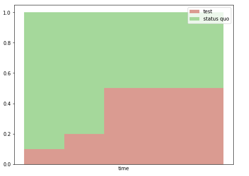
Example cohort allocation changes throughout an experiment
In this situation, we have multiple runs of the experiment with different cohort allocations in each run. This blog post will show how to properly analyze data from all runs of the experiment. We will discuss a common pitfall and show a way to avoid it. We will then frame this problem in the language of causal inference. This opens up numerous causal inference-based approaches (we survey a couple) that can yield further insight into our experiments.
Problems with changing cohort allocations
Comparing metrics between cohorts can get tricky if cohort allocations change over time. In this section, we show an example where failing to account for the changing cohort allocation can cause one to get misleading results.
For concreteness, suppose that we are trying to improve our home and local services experience, with a view towards getting more users to request a quote for their home projects on Yelp. The metric we are trying to optimize in this example is the conversion rate — what fraction of users visiting home and local services pages decides to actually request a quote.
We run an A/B test to ensure that the new experience improves conversion versus the status quo. We have two runs, one each in the winter and the spring; in the second run, we increase the fraction of traffic allocated to the test cohort from 10% to 50%. The cohort allocations and true per-cohort conversion rates in each experiment run are as in the table below.
| Time period | Experiment Run | Cohort | % of traffic assigned to cohort | Conversion Rate |
|---|---|---|---|---|
| Winter | 1 | Status Quo | 90% | 0.15 |
| Winter | 1 | Test | 10% | 0.15 |
| Spring | 2 | Status Quo | 50% | 0.30 |
| Spring | 2 | Test | 50% | 0.30 |
Notice that in this example, the conversion rate is higher in the spring. This can happen, for example, if home improvement projects are more popular in the spring than the winter, causing a higher fraction of visitors to use the Request a Quote feature. Importantly, there is no conversion rate difference between the two cohorts.
We will now simulate a dataset that one might obtain when running this experiment and show that if we fail to account for the changing cohort allocation, we will be misled to believe that the test cohort has a higher conversion rate.
Simulating experiment data
In our simulated dataset, we will have ten thousand samples for each experiment run. A given sample will include information about the experiment run, cohort, and whether a conversion occurred. The cohort is randomly assigned according to the experiment run’s cohort allocation. The conversion event is sampled according to the true conversion rate in the given experiment run and cohort.
import numpy as np
import pandas as pd

def simulate_data_for_experiment_run(
    total_num_samples: int,
    experiment_run: int,
    p_test: float,
    status_quo_conversion_rate: float,
    test_conversion_rate: float
):

    experiment_data = []
    for _ in range(total_num_samples):
        cohort = np.random.choice(
            ["status_quo", "test"],
            p=[1 - p_test, p_test]
        )
        if cohort == "status_quo":
            conversion_rate = status_quo_conversion_rate
        else:
            conversion_rate = test_conversion_rate

        # 1 if there is a conversion; 0 if there isn't
        conversion = np.random.binomial(n=1, p=conversion_rate)
        experiment_data.append(
            {
                'experiment_run': experiment_run,
                'cohort': cohort,
                'conversion': conversion
            }
        )

    return pd.DataFrame.from_records(experiment_data)
experiment_data = pd.concat(
    [
        simulate_data_for_experiment_run(
            total_num_samples=10000,
            experiment_run=1,
            p_test=0.1,
            status_quo_conversion_rate=0.15,
            test_conversion_rate=0.15,
        ),
        simulate_data_for_experiment_run(
            total_num_samples=10000,
            experiment_run=2,
            p_test=0.5,
            status_quo_conversion_rate=0.30,
            test_conversion_rate=0.30,
        ),
    ],
    axis=0,
)
Estimating the conversion rate
The most straightforward way one might try to estimate the per-cohort conversion rate is to take the mean of the conversion column for all samples in each cohort. Effectively, this gives the number of conversions per cohort divided by the total number of samples in the cohort.
def get_conversion_date_for_cohort(
    experiment_data: pd.DataFrame,
    cohort: str
):
    experiment_data_for_cohort = experiment_data[experiment_data.cohort == cohort]
    return experiment_data_for_cohort.conversion.mean()
get_conversion_date_for_cohort(experiment_data, "test")
0.2768492470627172

get_conversion_date_for_cohort(experiment_data, "status_quo")
0.20140431324783262
We observe a substantial difference between the conversion rate estimates for the status quo and test cohorts.
To get some intuition about whether it is statistically significant, let us create five thousand simulated datasets with the same parameters (cohort allocations and conversion rates). For each dataset, we will estimate conversion for the two cohorts, and look at the estimates’ distribution. The table below reports the mean and quantiles of the five thousand estimates of the status quo and test conversion rates. The table shows that the distributions in the estimated conversion rate for the two cohorts are very different, suggesting that the difference we observed is indeed statistically significant.
| Mean | 2.5th percentile | 50th percentile | 97.5th percentile | |
|---|---|---|---|---|
| Status Quo | 0.204 | 0.197 | 0.204 | 0.210 |
| Test | 0.275 | 0.246 | 0.275 | 0.287 |
Recall, however, that there is no conversion rate difference between the cohorts: for both experiment runs, the test and status quo cohorts have equal conversion rates. Thus, if we use the simple approach described above to analyze the experiment, we would be misled and think that the test cohort outperforms the status quo.
What is going on? What we are seeing is a consequence of the fact that the average conversion rates and cohort allocations both change between experiment runs. For the test cohort, the majority of samples come from the higher-conversion period of the second experiment run. The opposite is true for the status quo cohort. So, the calculated conversion rate is higher for the test cohort than for the status quo cohort.
(In fact, it is not hard to adapt this example so that the test cohort has a lower conversion rate than the status quo cohort in each experiment run, but a higher calculated conversion rate overall. In this case, we might be misled and release the test experience, despite the fact that it harms conversion. This phenomenon is an example of Simpson’s Paradox.)
A better way of calculating conversion rate
How do we correctly compare the conversion for the experiment cohorts? We first observe that the average conversion rate over the entire dataset is 0.225, the average of the conversion rates in each experimental run. (There are ten thousand samples in each run, so we can take a simple average. If the number of samples per run were different, we would instead calculate the overall conversion rate using a weighted average; the weights would be the number of samples in each experiment run.) Since the two cohorts have the same conversion rate, the method used for estimating it should arrive at this number for both (up to some statistical noise).
The previous method reported a higher conversion rate for the test cohort because it had disproportionately many samples from the second experiment run. To correct for this imbalance, let us instead try to calculate per-cohort conversion rates separately for each experiment run, and then combine them with a weighted average. This approach is implemented below:
def per_experiment_run_conversion_rate_estimator_for_cohort(
    data: pd.DataFrame,
    cohort: str,
    experiment_runs: List[int],
):
    data_for_cohort = data[data.cohort == cohort]

    conversion_rates = []
    total_num_samples = []

    for experiment_run in experiment_runs:
        conversion_rates.append(
            data_for_cohort[
                data_for_cohort.experiment_run == experiment_run
            ].conversion.mean()
        )
        total_num_samples.append(
            (data.experiment_run == experiment_run).sum()
        )

    return np.average(conversion_rates, weights=total_num_samples)
In the table below, we report statistics about conversion rate estimates on five thousand simulated datasets:
| Mean | 2.5th percentile | 50th percentile | 97.5th percentile | |
|---|---|---|---|---|
| Status Quo | 0.225 | 0.218 | 0.225 | 0.232 |
| Test | 0.225 | 0.213 | 0.225 | 0.238 |
We see that the estimates for the test and status quo conversion rates are close to the true value on average, and are close to each other.
In the rest of this blog post, we will provide a more theoretical justification for why this method, and another one based on regression, are appropriate for analyzing experiments where cohort allocations change over time. This will involve interpreting our problem in the language of causal inference.
An interpretation based on causality
The issues we faced when analyzing experiments with changing cohort sizes have a connection with causal inference. In this section, we will explore this connection, which will help us gain a better understanding of methods used to correctly calculate conversion rate (including the per-experiment run computation in the previous section).
What are we trying to measure?
We are trying to measure the causal effect on conversion from being in the test (versus the status quo) cohort (also known as the treatment effect). To do this, we imagine taking all the samples in our dataset. What fraction would convert if all of them were in the test cohort (call this YT)? What fraction would convert if all were in the status quo cohort (call this YSQ)? The difference between the two is the average treatment effect for the dataset.
Unfortunately, it is impossible to directly measure the average treatment effect as described above. Any given sample is in one cohort but not both, so it is impossible to know that sample’s outcome if it were in the other cohort. The calculation relies on some counterfactual data, e.g. for a sample in the status quo cohort, would it have converted had it been in the test cohort? This is known as the fundamental problem of causal inference.
However, we can use our samples to estimate the average treatment effect.
Estimating average treatment effect
The first attempt to estimate the average treatment effect was computing the average conversion rate per cohort. We computed the probability of conversion given that the cohort was test or status quo, and subtracted the two. We found that being in the test cohort was correlated with higher conversion. This correlation does not imply causation, however. The reason that being in the test cohort is correlated with conversion is that, given our cohort allocations, a user being in the test cohort means that they are more likely to be in the higher-conversion second experiment run.
Said another way, the experiment run is a confounding variable that produces a non-causal association between cohort and conversion. This is known as confounder bias. To properly estimate the causal effect of being in the test cohort, we have to control for the confounder. There are a number of standard ways of doing this in the causal inference literature (e.g. Section 3.2 of [1]).
Separate conversion rate calculations per confounder value
This approach tries to correct for confounder bias by computing per-cohort conversion rates separately for each value of the confounder (experiment run). To get the overall conversion rate for each cohort, we take a weighted average of the conversion rates per experiment run, with weights being the relative prevalence of each confounder value in the dataset. (See, for example, Equation 3.21 in [2].) This is equivalent to weighing by the total number of samples (test and status quo) in each experiment run. This gives estimates for YT and YSQ, and we can subtract them to get an estimate for the average treatment effect.
We did precisely this when we tried to properly calculate conversion rate per cohort
(using the per_experiment_run_conversion_rate_estimator_for_cohort function).
This approach makes sense because, for a given experiment run, the per-cohort calculation gives us an estimate of the conversion rate for that experiment run if all samples were in the given cohort (this relies on the fact that users are assigned at random to the status quo or test cohort). Then, the weighted average step gives us an estimate of what the conversion rate would be over the entire data set (all experiment runs).
Including confounding variable in a regression
Another approach for controlling for the confounder is to build a regression model for the outcome variable (conversion) as a function of the treatment variable (cohort, specifically a dummy variable encoding whether the sample is in the test cohort). If we simply regress conversion on the test cohort dummy variable, we will see a positive regression coefficient, which may lead us to conclude there is a positive treatment effect. However, in our running example — where the treatment effect is zero — there will be a positive coefficient just because being in the test cohort is correlated with conversion, which happens due to the presence of the confounder.
To fix this, we include the confounder as a predictor variable alongside the cohort. This will split the conversion effects that are due to the confounder and those due to being in the test cohort. The coefficient of the cohort variable will give us the average treatment effect.
Both the cohort and the experiment run are categorical variables, and we will encode them using dummy variables. For each categorical variable, we need one fewer dummy variable than the number of different values the variable can take. For our data with two cohorts and two experiment runs, the code below will create dummies for whether the user is in the test cohort and also for whether it is in the second experiment run.
import statsmodels.formula.api as smf
smf.ols(
    formula="conversion ~ C(cohort, Treatment('status_quo')) +  C(experiment_run)",
    data=experiment_data
).fit().summary()
This code uses the formula API in statsmodels. It stipulates that conversion is a linear function of cohort and experiment run. The C(·) notation encodes these variables as dummy variables.
The results are:
| Variable | Coefficient | Standard Error |
|---|---|---|
| Intercept | 0.1507 | 0.004 |
| User is in test cohort | 0.0073 | 0.007 |
| Second experiment run | 0.1427 | 0.006 |
The intercept term is approximately equal to the baseline conversion rate (in the first experiment run and status quo cohort), namely 0.15.
We see a close to zero effect from being in the test cohort; the coefficient is almost equal to its standard error. On the other hand, we see an approximately 0.15 effect from being in the second experiment run. Indeed, samples in that experiment run have a conversion of 0.3, which is 0.15 higher than the conversion rate in the first experiment run.
Example with non-zero treatment effect
We modified our running example such that the test cohort conversion rate was 0.05 higher in each experiment run than the status quo conversion rate, and tested out our two methods for computing average treatment effect.
| Time period | Experiment Run | Cohort | % of traffic assigned to cohort | Conversion Rate |
|---|---|---|---|---|
| Winter | 1 | Status Quo | 90% | 0.15 |
| Winter | 1 | Test | 10% | 0.20 |
| Spring | 2 | Status Quo | 50% | 0.30 |
| Spring | 2 | Test | 50% | 0.35 |
The overall conversion rates are 0.225 for the status quo cohort and 0.275 for the test cohort.
Separate conversion rate per confounder value
Running per_experiment_run_conversion_rate_estimator_for_cohort gives conversion rate estimates that are close to the actual values (0.225 and 0.275 for the status quo and test cohorts respectively).
Regression
The regression gives the following coefficients:
| Variable | Coefficient | Standard Error |
|---|---|---|
| Intercept | 0.1506 | 0.004 |
| User is in test cohort | 0.0567 | 0.007 |
| Second experiment run | 0.1431 | 0.007 |
As before, the coefficient for the variable encoding whether the user is in the test cohort approximates the true average treatment effect (0.05). The coefficient for the variable encoding the second experiment run is approximately 0.15, once again as expected — in the second experiment run, conversions are that amount higher.
Simulation study
To better understand the two methods for estimating average treatment effects and the advantages of each, we ran a simulation study. In this study, we produced a large number of datasets with the same parameters and looked at the distribution of average treatment effects estimated by the two methods.
We will take a look at a particular example:
- Two experiment runs with 1000 samples per run (ten times lower than in the previous datasets; this helps better illustrate the statistical noise in our estimates)
- Test cohort allocation is 10% and 50% in the two runs respectively
- The status quo conversion rates are 0.15 and 0.30 in the two experiment runs respectively
- The test cohort conversion rates are 0.20 and 0.35 (0.05 higher than the status quo conversion rates)
We produced a total of 5000 datasets, and hence estimated the treatment effect 5000 times for each method.
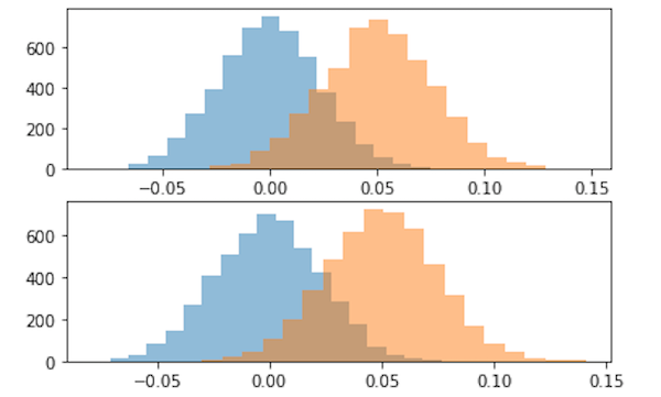
The orange graphs in the figure above are histograms of the estimated average treatment effect for the separate conversion rate estimation method (top) and the regression method (bottom). Both distributions have means close to 0.05, the true average treatment effect, and have very similar shapes. The graphs in blue are the estimated average treatment effects for datasets that are the same as above, but where the status quo and test cohorts have the same conversion rate in each experiment run. These distributions have means of close to 0 as expected, since the true treatment effect is 0.
We have run a number of simulation studies, and have found that the two methods for estimating average treatment effect perform similarly. Overall, we believe that the most important thing is not the precise method one uses, but that one is aware of confounder bias, and takes steps to correct for it.
Nevertheless, it is good to keep the regression method in one’s tool chest because it can be easier to use in many instances. For one, software packages such as statsmodels automatically compute standard errors for regression estimates. Additionally, with regression, it is fairly straightforward to analyze more complicated experiments, such as when there are multiple confounders. (One example is if cohort allocations within experiment runs were different for different geographical regions; in this case, geographical region would be an additional confounding variable.)
Conclusion
Analyzing experiments where cohort allocations change over time can get a little complicated. Simply looking at the outcome variable for samples in the status quo and test cohorts can cause misleading results, and different techniques, which control for the confounding variable, are needed. We hope that this blog post has raises awareness of this issue and provides some solutions.
Acknowledgements
- Billy Barbaro for originally making me aware of the issue discussed in this post.
- Alex Hsu and Shichao Ma for useful discussions and suggestions, which ultimately helped frame this causal inference interpretation of the problem.
- Blake Larkin and Eric Liu for carefully reading over this post and giving editorial suggestions.
References
- Joshua D. Angrist and Jörn-Steffen Pischke. Mostly Harmless Econometrics. Princeton University Press, 2008
- Judea Pearl. “Controlling Confounding Bias.” In Causality. Cambridge University Press, 2009 http://bayes.cs.ucla.edu/BOOK-2K/ch3-3.pdf
- Adam Kelleher. “A Technical Primer on Causality.” https://medium.com/@akelleh/a-technical-primer-on-causality-181db2575e41#.o1ztizosj
Become an Applied Scientist at Yelp
Want to impact our product with statistical modeling and experimentation improvements?
View Job