Fast Order Search Using Yelp’s Data Pipeline and Elasticsearch

-
Dmitriy Kunitskiy, Software Engineer
- Jun 1, 2018
Since its inception in 2013, Yelp has grown its transactions platform to tens of millions of orders. With this growth, it’s become slow and cumbersome to rely solely on MySQL for searching and retrieving user orders.
Transactions at Yelp are built around integrations with dozens of external fulfillment partners across different verticals, from food ordering to spa reservations. In most of these integrations, Yelp takes care of payment processing. Given this, the way we store order details prioritizes facilitating stateful order processing in a uniform way. However, other access patterns like finding popular orders by category or fetching a user’s full order history were not scaling well and were becoming pain points when writing new features. With this in mind, we decided to leverage Yelp’s real-time data pipeline to duplicate transactions data into Elasticsearch, which could provide the enhanced performance and powerful search capabilities we wanted, while being completely decoupled from the critical order processing workflow.
This blog post will look at the pipeline to ingest orders in near real-time into Elasticsearch, and the decisions we made along the way. In particular, we’ll look at Elasticpipe, a data infrastructure component we built with Apache Flink to sink any schematized Kafka topic into Elasticsearch. The correctness of Elasticpipe is validated by an auditing system that runs nightly and ensures all upstream records exist in Elasticsearch using an algorithm that requires only O(log(number of records)) queries. Finally, we’ll look at some client-side efforts to migrate to this more performant, eventually-consistent system.
The Problem
One example of what was wrong with our legacy order search backend was the deteriorating performance of the food order history page.

Food order history on iOS
Over time, the latency of this page started to increase, climbing to more than several seconds for some users. When we profiled the code, we saw that a lot of time (> 1s) was spent in database lookups:
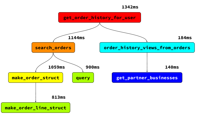
Simplified cProfile trace graph
Because order history information is split across multiple tables, each request required a join between the Order table, the OrderLine table (order lines are the individual items in an order, like “2 samosas”), the Address table, and the CancellationPolicy table. This was becoming expensive, especially considering that the order history page was not the only consumer of this data. More and more features across Yelp needed to access order history and, in many cases, the service calls to fetch it were some of the slowest made by clients.
We realized that we had been asking MySQL to do double duty. We needed:
- A relational data store with ACID guarantees to power the complicated finite state machine underlying order processing.
- A distributed key-value store for quickly retrieving order history that could be used in latency-sensitive, high-traffic applications.
On top of this, we became increasingly interested in having a backend that acts as a general purpose search engine with full text search, allowing us to do things like find the most commonly ordered dishes for a restaurant, or even the most popular burger in a particular area.
Although some of these problems, like speeding up the order history page, could have been solved by more aggressive MySQL indexing or materialized views, we knew these would be temporary solutions that wouldn’t solve our needs more broadly and wouldn’t grow with our future product goals. It became clear that we’d need a different tool to solve this new class of problems.
New Datastore
After considering a few alternative NoSQL datastores, we chose Elasticsearch because it could accomodate all of our use cases, from retrieving a single user’s order history, to full text search over order items, to fast geolocation queries. It is also widely deployed at Yelp as the backend for new search engines, so a lot of tooling and infrastructure for it already exists. The most attractive attribute was the flexibility to make new queries that we may not have anticipated when first designing the data model - something that’s much more difficult with datastores like Cassandra.
The next step was to determine the schema of the denormalized order document that we’d want to store in Elasticsearch. Although it sounds trivial, it required surveying the current clients and thinking of possible future uses cases to determine the subset of fields that would form the denormalized order from over 15 tables that store information pertaining to orders. The tradeoffs here are clear. On one hand, there was no cost to adding fields, especially if we may need them in the future. On the other hand, we don’t want to bloat the order object with unnecessary information, since:
- Each new field makes the Elasticsearch document schema more brittle and sensitive to changes in the MySQL schema.
- Adding a field that requires joining on a new database table in constructing the order document adds latency to the pipeline.
- We don’t want requests to Elasticsearch to return very large response bodies, requiring us to paginate them when we might not otherwise have needed to.
After some discussion, we developed a schema that includes the high level order state, all the order lines, the user id, information about how the user entered the order flow, plus some high level partner details. We chose to exclude details of the business itself, all details of the user aside from the delivery address, and any details about the payment processing.
Change Replication Pipeline
With the datastore and schema determined, the next question would be how we’d funnel our MySQL data into it. The most straightforward approach might be a batch that periodically queries MySQL for new orders and uses the Elasticsearch REST API to insert them. This has its share of problems, including:
- The latency between an order being placed and being picked up by the batch.
- Lack of clarity for how to track updated orders since the last batch run without polluting our MySQL schemas with new flags to mark unflushed updates.
- Inability to quickly rebuild our data in Elasticsearch from scratch in the case of data loss or corruption.
Another solution we considered was writing into Elasticsearch as a part of order processing anytime an order enters a terminal state such as “completed” or “cancelled”. As part of this solution, we would also run a one-time backfill batch to insert historical orders. The most significant drawback was what to do if the write request to Elasticsearch failed. Failing or stalling order processing is clearly unacceptable, but the alternative of ignoring the write failure results in missing data in Elasticsearch.
Fortunately, we didn’t have to use these ad-hoc solutions and were able to leverage Yelp’s realtime data pipeline, which persists incoming MySQL data to Kafka by scraping MySQL binary logs. This allowed us to build an asynchronous processing pipeline for Elasticsearch writes out of band with order processing itself.
One new difficulty that presented itself was how to make sense of many independent Kafka streams of change events, with each table’s changes written to a different Kafka topic. As mentioned above, orders go through multiple intermediary states, with state changes reflected across multiple tables and written out in large database transactions.
As an example: you’re ordering a pizza, but immediately after ordering you decide to add extra toppings and deliver to a friend’s address. In our order processing state machine, credit card transactions are processed asynchronously. An update like this is persisted in MySQL as a new Order row with a “pending” status and foreign key to a new Address row, in addition to a new OrderLine row for the new pizza. In this way, the history of an order is maintained as a linked list, with the tail of the list being the most current order. If the credit card transaction succeeds, yet another Order row will be created in a “completed” state - if it fails, the order will be rolled back by adding a new row which duplicates the order state prior to the attempted update. Here’s how just the first part of this operation, the creation of new Order row in a “pending” state, would look when seen as a series of independent events in the data pipeline:
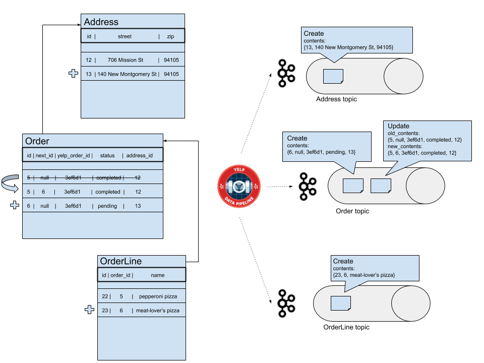
Yelp's data pipeline persists MySQL writes to Kafka
Since each high level update can result in dozens of data pipeline events, reconstructing high level order updates and materializing them at the appropriate times is a challenging problem. We considered two approaches:
- Independently Insert Each Table Stream
- Select One of the Table Streams as a Signal of High Level Changes
Independently Insert Each Table Stream
The first approach was to run independent processes for inserting events from each table’s data pipeline topic. Given that we wanted a single Elasticsearch index of order documents, a process inserting events from a supporting table (like Address) would need to query to find which orders would be affected by an event and then update those orders. The most concerning challenge with this approach is the need to control the relative order in which events are inserted into Elasticsearch. Taking the example of related address and order events in the above diagram, we would need an order event to be inserted first, so that the address event has a corresponding order to be upserted into.
Another difficulty with this approach is more subtle: resulting records in Elasticsearch may never have existed in MySQL. Consider an incoming update that altered both an order’s address and order lines in one database transaction. Because of the separate processing of each stream, an order in Elasticsearch would reflect those changes in two separate steps. The consequence is that a document read from Elasticsearch after one update has been applied but not the other is one that never existed in MySQL.
Select One of the Table Streams as a Signal of High Level Changes
The second approach is a result of analyzing our data model and finding a common pattern in high level order changes: ultimately, they make a change to the Order table.
In database terminology, our schema was a Snowflake and Order was a Fact table. Meaning that, if we could figure out how to map events from the Order table’s data pipeline stream to high level operations on the order, we could watch for changes just to this table. When seeing a row created or updated event, we could first check whether or not the row was for an order in a finalized state. If it was, we could query the database for this row’s foreign keys and use that to create a full denormalized order document, ready to insert into Elasticsearch.
Ultimately we chose this approach because it was simple and eliminated the problem of partial updates from MySQL being inserted in Elasticsearch. However, this has some downsides:
- Not easily generalizable. If we introduce an update pattern which affects a Dimension table without affecting the Fact table, this mechanism wouldn’t work.
- Adds extra read load on the database. Since we don’t utilize the row contents in data pipeline messages except to filter out rows in intermediary stages, each order update ending in a final state results in additional reads to create the order document.
The approach led us to design an order ingestion pipeline with two main steps. The first consumes data pipeline events from the Order table and constructs denormalized order documents. These are written to a downstream Kafka topic, which is then read by the second step that writes them into Elasticsearch. This architecture is shown in the following schematic:
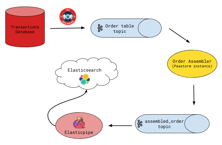
Ingestion pipeline
Order Assembler
The order assembler is a Paastorm instance (our in-house stream processor) which consumes the Order table’s data pipeline stream, reads the required additional fields from the database, and constructs order documents for insertion into Elasticsearch. Since we don’t care about maintaining orders in intermediary states, the assembler skips events for order rows in transient states. The resulting documents are written to an intermediary Kafka topic, which we refer to as the assembled_order topic. Having a two-step design with an intermediary topic in between allows us to separate the concerns of assembling the denormalized order in the representation we want and writing it to Elasticsearch into isolated parts, with the latter done by Elasticpipe (described below).
Additionally, setting infinite retention on this intermediary topic turns out to be an effective backup in the case of data loss or corruption in Elasticsearch. The assembled_order topic cuts down disaster recovery time by an order of magnitude because writing the entire assembled_order topic to Elasticsearch is a lot faster than recreating that topic from events in the data pipeline Order table stream (a few hours versus a few days). This is because the order assembler processes records one at a time, requiring a database read across multiple tables for every order, whereas sinking records to Elasticsearch over the network can be done in large batches. Lastly, the assembled_order topic is log compacted by Kafka, allowing us to retain only the last order version for each order (although we don’t assemble intermediary order states, an order can go through multiple final states, such as being completed, then updated, and then cancelled).
Elasticpipe
The last step of the pipeline is a data connector we wrote using Apache Flink. Rather than writing a single-purpose app for order search, we made one that could work with any schematized Kafka topic. Elasticpipe solves the problem of writing all records from a schematized Kafka topic to an Elasticsearch index.
Because Flink comes with an Elasticsearch connector that takes care of generating bulk requests and handling API failures, the only remaining parts to solve were:
- Bridging the possible gap between the Elasticsearch mapping and the schema of the topic we wanted to sink
- Forming idempotent insert requests
- Implementing offset recovery on restart
In dealing with the potential for divergence between the topic schema and the Elasticsearch mapping, we get help from the following Elasticsearch feature: type coercion. This means that types in the mapping can differ somewhat from those of the Avro schema (we use Avro to serialize Kafka messages), and Elasticsearch will do the conversion at write time.
When starting to sink a new topic, we require a developer to manually create a corresponding index in Elasticsearch with a compatible mapping. We also require the mapping to include an extra field to hold document metadata which gets added to every document. For example, an order record is actually indexed as:
{
	"order": {
		"total_price": 17.95,
		"user_id": 12345,
		"order_lines": [
			{"name": "meat-lover’s pizza",
			 "description": "sausage, pepperoni and pancetta in a hearty tomato sauce",
			...
			}
		]
		...
	}
	"metadata": {
		"cluster_name": "uswest2",
		"cluster_type": "datapipe",
		"topic": "assembled_order",
		"partition": 0,
		"offset": 55,
		"doc_id": "ab12cd34ab12cd34ab12cd34ab12cd34"
	}
}
Storing this extra state in Elasticsearch allows Elasticpipe to do stateless offset recovery on restarts and helps with auditing.
Currently, the index creation process is done manually. Since setting the options for how fields are stored and analyzed is critical in obtaining utility from Elasticsearch, we are okay leaving this to the developer for now. However, this process is also prone to human error so we’re considering writing a command-line script that will generate a “starter” mapping from a topic’s Avro schema which a developer could then tweak to suit his/her needs. Schema auto-generation is something we commonly do in other data connectors and have found it valuable in reducing uncertainty about how different datastore schemas interact. For Elasticpipe, we could generate a starter mapping using a type translation table like:
| Avro type | Elasticsearch type |
|---|---|
| boolean | boolean |
| int | integer |
| long | long |
| float | float |
| double | double |
| bytes | keyword |
| string | text |
| array | nested |
| map | object |
Of these, the array type is the most interesting. By default, arrays don’t work as expected in the Elasticsearch data model because array item fields are dissociated from each other. We faced this problem in the context of order lines, which are an array of the items in an order. Had we used the default behavior, we would have been unable to query for “orders containing 3 meat-lover’s pizzas”, for instance, because the quantity field and name field of an order line item would no longer be associated with each other. Instead, we chose the alternative, which is the “nested” datatype. It creates new documents for each array element, and transparently joins them at query time. The downside is that this is more resource intensive, especially for high cardinality arrays.
Turning to the question of how to structure insert requests, we chose to make every request an upsert based on the document id, where the id is the same as the message key in the Kafka topic. This ensures that all index requests are idempotent and that we can replay the Kafka topic from any offset. What about unkeyed Kafka topics? Consider a topic that records some client-side event (i.e. button-clicks). If a developer decides to pipe these to Elasticsearch, we still need inserts to be idempotent. To accomplish this, records from unkeyed topics are inserted under a pseudo-key, which is a hash of the message’s Kafka position info - that is, a hash over the cluster info, topic name, partition, and offset.
Lastly, we needed a way for Elasticpipe to pick up where it left off after a restart. One of the strengths of Flink is its built-in state-saving mechanism, which is extended to the Elasticsearch connector. However, saving and reading state, especially on an eventually consistent store like Amazon S3, extends the surface area for failure. In this case, we saw that we could make the application stateless by querying Elasticsearch on startup to find the last seen offset for a topic. Since the last executed bulk write could have succeeded only partially, and since writes are idempotent, we actually restart at an offset which is the max seen in Elasticsearch minus the bulk write size. In practice, this way of doing offset recovery has proven very reliable.
Auditor
With a new component like Elasticpipe, we wanted to build confidence in its correctness, so we set up an auditing mechanism to ensure that it’s not silently skipping records without our knowledge. Additionally, Elasticsearch doesn’t make ACID guarantees and can lose data in the case of network partitions so we wanted to periodically ensure that our index still has all the records we expect if we plan to rely on it as a NoSQL database. Having such an auditor allows us to avoid periodic full re-indexing, a common but heavy handed solution to the potential for data loss in Elasticsearch.
The most basic approach of scanning the upstream topic and checking that every document exists in Elasticsearch, even in bulk, would be as slow as a full reindex of the upstream topic. We wanted a more performant solution that would scale more favorably than O(n) in terms of number of network requests per upstream document.
One of the existing ideas for this problem is using histogram aggregations to find missing records. However, this doesn’t work when your document ids are uuids instead of continuous integer ranges. So, for our application, we developed the following auditing algorithm which uses binary search to find missing documents:
- Get the upstream topic’s low and high watermarks
- Get all message keys in the upstream topic between the low and high watermark
- De-duplicate and sort the keys into an in-memory array
- Sleep for Elasticpipe’s max bulk-write time interval, to allow for documents to be flushed
- Query Elasticsearch to find possibly-missing keys, which are those that don’t exist in the index under the restriction that we only query for records whose offset (which is part of the metadata we include with each document) is between the low and high watermarks from step 1. (More on this below)
- Without the high watermark offset limit, query to find which of the possibly-missing documents are actually missing. This is the final result.
Once we have a sorted and deduped list of all the document ids which should exist in Elasticsearch by scanning the upstream topic (after step 3), we can use binary search to find the possibly missing documents with O(log(n)) range queries, which Elasticsearch supports both over strings and numeric types. (A word of warning: versions over 5.0 of Elasticsearch do not support range queries over the _id, which is why we have duplicated the id in the document body explicitly as a field in the metadata.)
For example, if the low and high watermarks are L and H, the list of keys has n documents, with the first and last (in lexicographic order) documents having keys k1 and k2, respectively, we can query Elasticsearch for the number of documents between k1 and k2 with an offset between L and H. If the result is equal to n, we’re done. If it’s less than n, we can split the list into a left and right half and binary search recursively until either the number of documents in the range matches what we expected, or all the documents in the range are missing (typically when the range reaches size 1).
At this point, why are the documents we find only “possibly missing”? Because some documents in the list from step 3 could have been updated while the auditing is underway, which would get upserted into Elasticsearch with an offset higher than H. Because these documents aren’t actually missing, this requires a final step to explicitly find which of the possibly missing documents is actually missing by querying for the possibly missing document ids without the high watermark offset limit. This two-step process is necessary to ensure that brand new documents added to the index after auditing has started don’t pollute the range queries we make, causing us to undercount missing documents. The diagram below, which visualizes documents in Elasticsearch sorted by offset, explains this further:
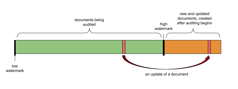
Documents being audited, ordered by increasing offset. The arrow is an upsert that happens while the auditor is running.
Although the auditing algorithm doesn’t detect all possible failure cases, such as corruptions inside document bodies, running it daily gives users a good degree of confidence in the continuous integrity of data in their indices.
Eventual Consistency
Lastly, let’s look at some difficulties of migrating existing applications that had previously been querying MySQL to an eventually-consistent data store.
The difficulty stems from the lag of 10-20 seconds between a change being committed in a master database and that change being visible in Elasticsearch queries. The lag is primarily driven by the bulk writes to Kafka of the data pipeline MySQL binary log parser. These bulk writes ensure max throughput when processing hundreds of thousands of writes per second, but it means that data pipeline table streams, and therefore the order search pipeline, is always behind the truth of what has been committed in MySQL.
We’ve found two strategies for making a migration. The first is dark-launching, which entails sending requests to both MySQL and Elasticsearch at the same time for a period of a few days to a few weeks and then comparing their output. If we find only a negligible number of requests get differing results, and those differences do not adversely affect users, we can feel confident about making the switch. The second is rewriting clients to be aware that the data they receive might be stale. This strategy requires more work, but is superior because the clients are in the best position to take mitigating actions. One example is the new order history client in Yelp’s iOS and Android apps, which now keeps track of recent orders placed using the app, and sends the id of the most recent order to the backend. The backend queries Elasticsearch and, in the case that the most recent order is not found, will make a supplementary query to MySQL. This way we still get low latency times for the vast majority of queries, while also ensuring that the pipeline latency does not result in users not seeing their most recent order.
Acknowledgements
Thanks to Anthony Luu, Matthew Ess, Jerry Zhao, Mostafa Rokooie, Taras Anatsko, and Vipul Singh, who contributed to this project, in addition to Yelp’s Data Pipeline and Stream Processing teams for their advice and support.
Read the posts in the series:
- Billions of Messages a Day - Yelp's Real-time Data Pipeline
- Streaming MySQL tables in real-time to Kafka
- More Than Just a Schema Store
- PaaStorm: A Streaming Processor
- Data Pipeline: Salesforce Connector
- Streaming Messages from Kafka into Redshift in near Real-Time
- Open-Sourcing Yelp's Data Pipeline
- Making 30x Performance Improvements on Yelp’s MySQLStreamer
- Black-Box Auditing: Verifying End-to-End Replication Integrity between MySQL and Redshift
- Fast Order Search Using Yelp’s Data Pipeline and Elasticsearch
- Joinery: A Tale of Un-Windowed Joins
- Streaming Cassandra into Kafka in (Near) Real-Time: Part 1
- Streaming Cassandra into Kafka in (Near) Real-Time: Part 2
Become an Engineer at Yelp
Want to work on challenges that span applications and infrastructure? Apply below!
View Job